I always thought I loved learning. The thought of knowing a lot excites me. So, for years I tried to come up with better ways to do it. I read many books and tried many techniques. I set schedules, made mind maps and read up on the neuroscience. Yet I never learned as much as I wanted to, and it remained difficult. Want to know topos theory? Find the best books and study the hell out of them, with all of these cool techniques I’ve learned. But nearly every book got abandoned. The same with papers. “If you want to get to the cutting edge, you have to read all the papers!” This went even worse than the books…
I blamed myself for a lack of discipline, or reasoned that perhaps this particular field isn’t for me. I felt that I wasn’t an expert in anything. But the desire to learn remained – or so I thought.
It took many decades of a futile cycle to find out the truth. I would make a commitment to some area, gather the books and papers and get to work, and it would fizzle out after a while. Some time later, I would repeat this with some other topic, with greater determination and vowing that this time I would see it through. This went on for years!
I love mathematics, so why did I not love studying it? Perhaps I was broken in some way, simply too weak to ever be good at the thing I love. Then I noticed some things about myself. Sometimes, I could spend hours, weeks or months pondering a mathematical thing, and it gave me great pleasure. It did not feel like discipline, or work. It was natural to do, and I hated anyone or anything interrupting this reverie.
Finally, the truth dawned: I do not love learning – if you consider effective learning as the rapid acquisition of information with the ability to provide an accurate representation of it at a later stage. What I do love is figuring stuff out! That’s why the books didn’t do it for me. I could read about differentiable manifolds all day long, doing all the exercises, and not be able to tell you a damn thing about them a week later. That is because I was trying to satisfy the author’s expectations (like you would a teacher’s) instead of getting it to make sense for me.
Instead of studying some mathematical topic now, I look for something that really tickles me. Something I want to understand. “That’s interesting – why does this thing do that?” I’ll try to come up with an answer based on my existing knowledge for a while, then realize it is hopelessly insufficient. Then I’ll go hunting for an explanation – scanning books, watching YouTube videos, doing Google searches (I tend to avoid AI for this, but I do use it for some other things). “Hmmm – it looks like I can’t understand what’s going on here without knowing more about manifolds…” The mistake would then be to grab a book on manifolds and try to study it. I want to know just enough to answer the question. Invariably though, that subject itself will interest me, because I would want to know why it is important in this case, and that isn’t really possible without knowing why it is important in other cases. I’ll often going into the history or applications of it. Then I would start pondering. Why were manifolds invented? Why would they come in handy? Who came up with them, and why? What kind of thing is not a manifold? How does a manifold relate to the idea of a derivative? But don’t get too deep into this rabbit hole; go back to the original question.
The reason I hadn’t done this more often is because I thought it was too slow. Taking a week to think about the point of a manifold is a week I could have spent going through an entire chapter in a book! Instead, this prejudice against pondering actually slowed me down, because I never developed a good internal representation of the concept, but plowed ahead with the technical stuff before I was ready for it. I would then get lost in the minutiae, and lose interest because I was trying to run before I could walk.
There are those that can happily plow through a book on Lie algebras and read it from start to finish. I am not one of those people. I cannot learn for the sake of learning, I need to have a compelling mystery which I have to solve, and I need to put together clues my way instead of following someone else’s teaching. This is the only way I can understand deeply, and remember well. I need to give myself the time to do this, instead of chasing results. It may not seem like it, but if you’re anything like me, prioritizing depth instead of speed will actually make you faster.
Not much help if you have a calculus exam tomorrow, though…
 ,
, is the permittivity of free space and
  is the magnetic permeability.
 ? Since force is measured in Newton (
 ), charge in Coulomb (
 ), we know immediately that Coulomb’s constant has units of
 .
. , which means we can express permittivity in the units
 ? Permittivity is supposed to measure the “polarizability” of a material: a low value means the material polarizes less easily. In order to polarize something, work has to be done, so energy is required, which means part of the potential energy due to two charges is used for the polarization. Therefore, a part of the potential energy is stored in the polarized medium, and the electric field is decreased. A high permittivity leads to a low field intensity, as is evident in a good conductor, which has almost no field inside the substance.
  ,
, 

 represents inductance and

 and
and  are easy to compute, we have a quicker way to compute the Fourier coefficients of the convolution, which doesn’t involve computing some ostensibly more difficult integrals. Which requires us to answer the question: why do we want to calculate the convolution in the first place?


 ,
,  ,
,  and
and  . This implies that

 . The contribution of a frequency
  to
to  (in other words, the
 when
when  ,
, , we need to multiply
  and
and  for all values of
  , which leads to our definition.
 the function obtained by integrating

 , we see there is nothing in the above expression that cannot be generalised to any positive real number (we’ll stick to these for now, lest we get lost too early). Supposing
  , we define
 , the above does not work. Instead, we cheat a little by making the lower bound finite:
 used, but we gain the ability to integrate more functions this way. So, we have a fractional integral, but how do we get to the derivative? By remembering the above relation between derivative and integral, we can set
 , which indicates that this is a derivative of order
  -th derivative of a simple function, say
  and the second is the constant 2, the

 is easy enough to compute (use a substitution to turn it into a Gaussian) and is equal to
  . The rest of the integral is not too difficult either – just use the substitution
  . This gives us


 , and suppose the original dice has probability function
  . What if the probabilities are not equal (the die is weighted)?
 and
and  . We can try to make this work by analogy (which is how most mathematics is done). Suppose we have functions
 are random variables over the reals with reader’s choice of appropriate
  -algebra.) We set

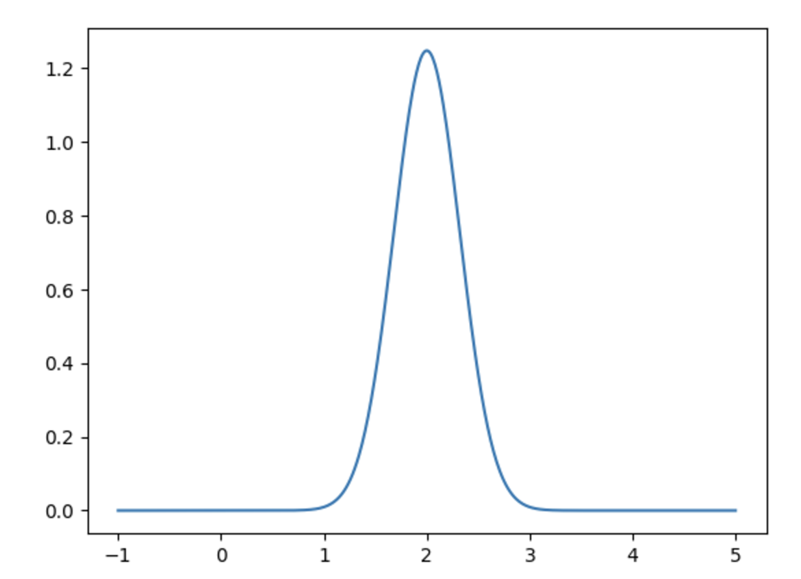
 and
and  , we get the following graphs for the density functions:


 and, by necessity,
  . Letting the hypotenuse be 1, the side adjacent to
  and the remaining side (necessarily) being
  , we have that


 . By replacing
  with
with  , we get

 , we can immediately get Fourier’s identity:

 is some function of distance,
  . We’re not going to discuss how this equation came about and are just going to accept it as it is. There’s a good (but short) post on some of the history
  , in one time variable
  and one space variable
 ![z \in [0,L]](https://s0.wp.com/latex.php?latex=z+%5Cin+%5B0%2CL%5D&bg=ffffff&fg=4c4c4c&s=0&c=20201002) . The given boundary and initial conditions are
. The given boundary and initial conditions are  and
and  . How to formulate these conditions in FEniCS?
  was specified earlier in the code, as usual. In my case, I wanted
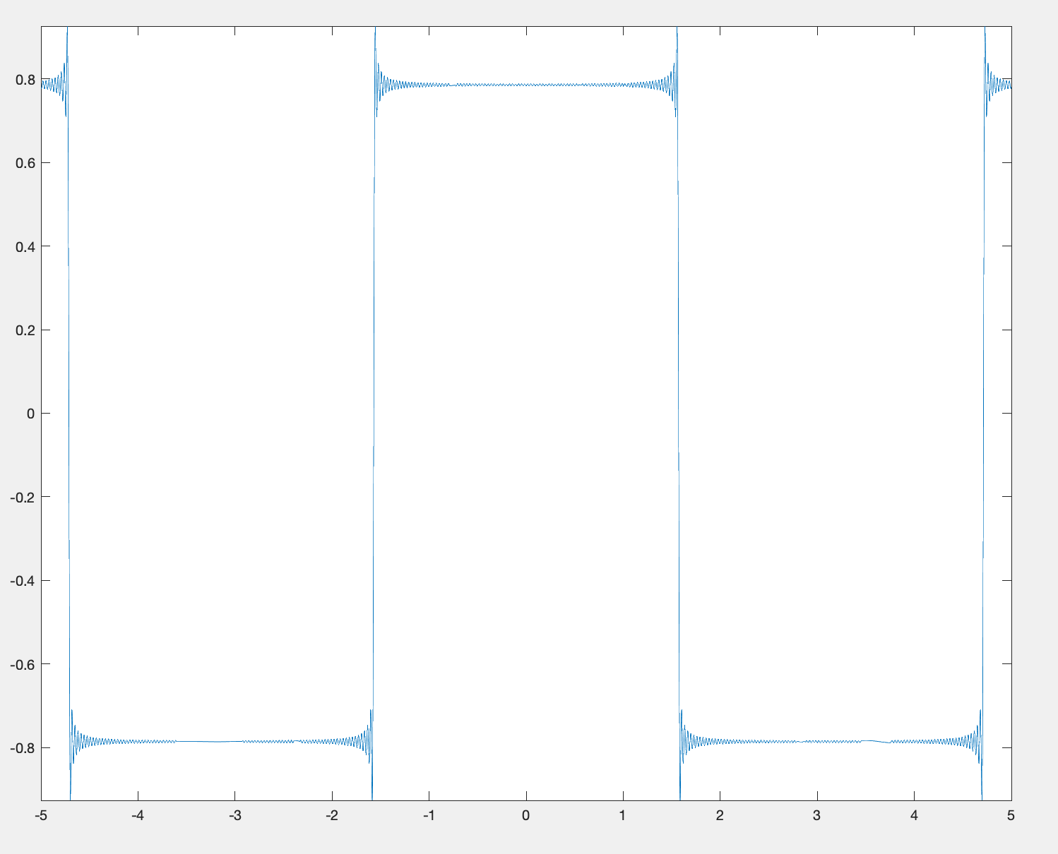
 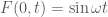 , so I set
 ![g(x[0],t) = (1-x[0])*\sin \omega t](https://s0.wp.com/latex.php?latex=g%28x%5B0%5D%2Ct%29+%3D+%281-x%5B0%5D%29%2A%5Csin+%5Comega+t&bg=ffffff&fg=4c4c4c&s=0&c=20201002) . What about the initial condition
. What about the initial condition  in
in  , it is indeed specified. If we want to add Neumann boundary conditions, we don’t need to do anything more – they are included by default.